Brain Age from MRI: from a biased regressor to a biomarker for Alzheimer's disease and headache

TL;DR

Q: Can a deep network estimate "brain age" from a single T1-weighted MRI accurately enough, and without systematic bias, that the gap between brain age and chronological age becomes a usable marker of Alzheimer's disease and headache disorders?

Gap: Brain age has almost always been posed as regression. Regression to the mean makes such models over-estimate the age of young brains and under-estimate old ones, and deep regressors reported 4–5 year errors on healthy cohorts. Both problems blunt the signal exactly where it matters (AD patients are 50+). Post-hoc "bias correction" with chronological age papers over the issue and makes downstream group comparisons questionable.
Method: Re-cast brain age as ordinal classification over integer ages 8–95, and add an ORDER loss (ORdinal Distance Encoded Regularization) that pushes penultimate-layer features apart in proportion to the age difference between samples in a mini-batch. Predicted age is the softmax expectation \(\sum_k k\,P(\text{age}=k)\). A 3D ResNet-18 is trained on 7,377 healthy scans from five public cohorts, then frozen and applied to clinical cohorts.
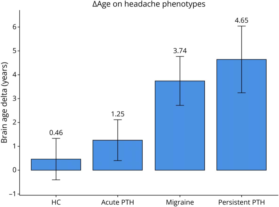
Results: MAE drops from 3.93 (MSE regression) to 2.56 years; the ordinality of the learned feature space is restored (0.98 vs 0.31 for plain cross-entropy) and systematic bias in the youngest and oldest subjects shrinks from +3.4/−4.2 to +0.1/−2.5 years. On 1,584 ADNI scans the brain-age gap rises monotonically HC < HC→MCI < stable MCI < MCI→AD < AD (r = 0.98). On 378 Mayo Clinic participants, the gap is 0.46 y in controls, 1.25 y in acute post-traumatic headache (APTH), 3.74 y in migraine and 4.65 y in persistent PTH; and within APTH, people whose headache was still present at 6 months had a baseline gap of 3.46 y versus 1.28 y for those who recovered by 3 months.

One-line summary: treating age as an ordered set of classes rather than a continuous target removes most of the regression-to-the-mean bias in brain age, and the resulting \(\Delta_{\text{age}}\) tracks disease stage in AD and predicts headache persistence after concussion.

00 · Primer

What brain age is, and why a two-year error matters

Everyone ages at the same rate chronologically, but brains do not. Genetics, environment and underlying neurological conditions push the structural trajectory of an individual brain ahead of or behind the population norm. Brain age is the age at which a person's MRI would be typical. The quantity of interest is the gap11Called BrainAGE (Brain Age Gap Estimate) by Franke et al.[8], brain-PAD elsewhere, and \(\Delta_{\text{age}}\) in our Neurology paper. I use \(\Delta_{\text{age}}\) here.

\[\Delta_{\text{age}} = \underbrace{\hat a}_{\text{predicted brain age}} - \underbrace{a}_{\text{chronological age}}\]

A positive \(\Delta_{\text{age}}\) means an older-looking brain. Elevated values have been linked to mortality[11], traumatic brain injury[12], and the Alzheimer's continuum. The idea is attractive because it collapses a whole 3D image into a single, interpretable number in years, and because the model only ever needs to be trained on healthy people. Disease is detected as deviation from normal ageing, not learned from labelled patients.

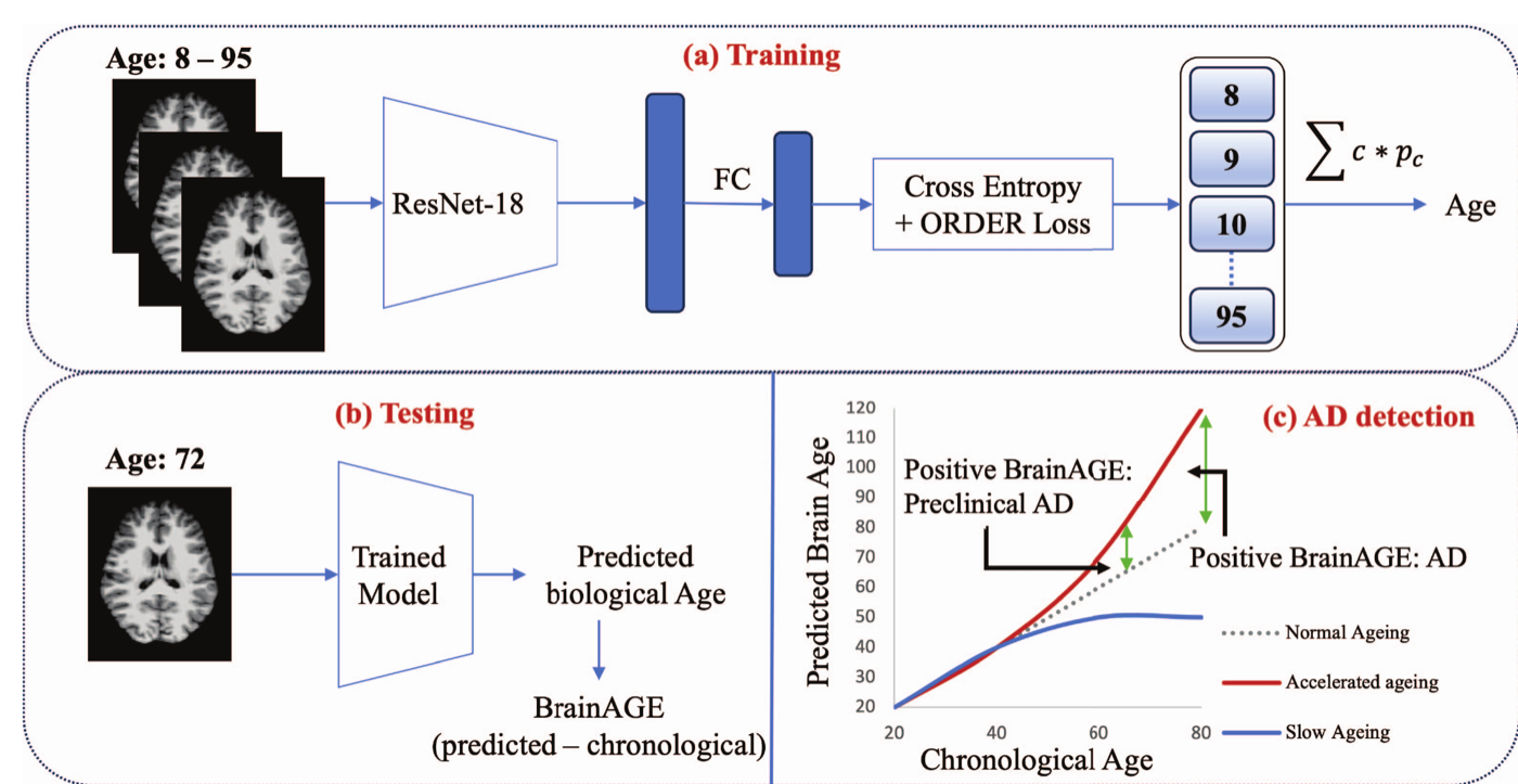
Overview of the brain age prediction framework: training a 3D ResNet-18 with cross-entropy plus ORDER loss on ages 8–95, testing to obtain BrainAGE, and the AD detection trajectory plot — Figure 1. The framework. (a) A 3D ResNet-18 is trained on the lifespan cohort with cross-entropy + ORDER loss; age is the expectation of the class probabilities. (b) At inference, \(\Delta_{\text{age}}\) = predicted − chronological. (c) Why it matters for AD: in the preclinical stage a person is cognitively normal, but accelerated ageing (red) has already begun to diverge from the normal trajectory (grey). Adapted from [1].

That last point sets the bar. Preclinical AD, the window where intervention is most plausible, produces subtle differences: a year or two of extra ageing. If the model's own error on healthy people is 4–5 years, and worse, if that error is systematically signed by age, the clinical signal disappears into it.

01 · The problem

Regression to the mean is baked into the formulation

Brain age models consistently over-estimate the age of young subjects and under-estimate old ones. The literature debated whether this came from the learning algorithm, imbalanced age sampling, or scanner heterogeneity, and Liang et al.[14] showed it is none of those. It is regression to the mean: a model minimising squared error lowers its loss by shrinking extreme predictions toward the cohort mean. Our claim in [1] is that the bias is therefore inherent to posing brain age as regression.

The standard fix is post-hoc: regress \(\Delta_{\text{age}}\) (or predicted age) on chronological age and subtract the fitted slope and intercept. That has three problems. It increases the variance of the corrected \(\Delta_{\text{age}}\); it breaks when the test cohort's age range differs from training; and, most fundamentally, explicitly controlling for age in a two-step pipeline makes any downstream analysis of "age-related" effects circular. A 2023 analysis by Zhang and colleagues showed that linear and quadratic corrections push the average gap to zero while making the bias for same-age subjects worse.

Our first attempt[6] was a plain 3D ResNet regressor. It was accurate for its time (MAE 3.76 y, R² 0.93, 10-fold CV) and already ordered the ADNI groups correctly, but the signed bias was obvious in the youngest and oldest subjects. Swapping the regressor for a classifier was the first thing that actually moved the bias[5]:

Table 1 · Regression vs classification on the same held-out healthy test set (AAIC 2023 [5])
Formulation	MAE (y)	R²	Mean \(\Delta_{\text{age}}\), age < 30	Mean \(\Delta_{\text{age}}\), age > 70
Regression (MSE)	3.93	0.90	+3.17	−2.49
Classification (CE + mean–variance)	2.41	0.96	+0.20	−0.97

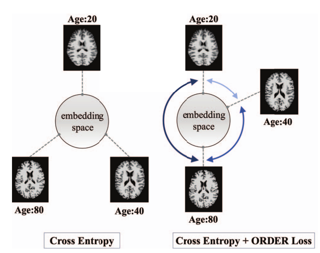
Why would discretising a continuous target help? Zhang et al.[9] argue that classification learns high-entropy feature representations: embeddings spread out across the space rather than collapsing onto a one-dimensional manifold. The same effect shows up in face-age estimation, depth estimation and crowd counting. But cross-entropy has its own flaw for an ordinal target: it treats every wrong class as equally wrong. A 53-year-old predicted as 52 is penalised exactly like one predicted as 21. The ordinal structure of age, which is the whole reason regression was chosen in the first place, is lost.

02 · Method

ORDER: ordinal classification with distance regularization

The goal is to keep the diverse, high-entropy features that cross-entropy produces while forcing them to respect age order. ORDER does this with a term computed on the penultimate-layer features within each mini-batch. For sample \(i\) with L2-normalised feature \(\bar x_i\), define

\[\phi(x_i) = \frac{1}{N-1}\sum_{j \ne i} \lvert y_i - y_j \rvert \; \lVert \bar x_i - \bar x_j \rVert_1\]

i.e. the Manhattan distance between two samples' features, weighted by the absolute difference between their ages. Adding \(\phi(x_i)\) to the target logit \(z_i = W_{y_i}^{\top} x_i\) inside the cross-entropy and expanding gives a loss that decomposes cleanly:

\[\begin{aligned}\mathcal{L}_T &= -\frac{1}{N}\sum_{i=1}^{N}\log\frac{e^{\,z_i + \phi(x_i)}}{\sum_{c} e^{\,W_c^{\top} x_i}} \\[6pt] &= \mathcal{L}_{\text{CE}} \;\underbrace{-\;\frac{1}{N(N-1)}\sum_{i}\sum_{j\ne i}\lvert y_i - y_j\rvert\,\lVert \bar x_i - \bar x_j\rVert_1}_{\mathcal{L}_{\text{ORDER}}}\end{aligned}\]

Minimising \(\mathcal{L}_{\text{ORDER}}\) maximises inter-sample feature distance in proportion to age difference: two 20-year-olds may sit close together, a 20- and an 80-year-old must not. Figure 2 is the cartoon version.

Cartoon of embedding space under cross-entropy versus cross-entropy with ORDER loss, showing scans aged 20, 40 and 80 spaced in proportion to age difference — Figure 2. Cross-entropy alone (left) spreads embeddings out but ignores label order. With ORDER (right), scans aged 20, 40 and 80 are pushed apart by amounts proportional to their age differences. From [1].

Why Manhattan?

In high dimensions (512-d here) Euclidean distances concentrate: the ratio of nearest to farthest neighbour approaches 1[15], which is part of why a classifier cannot "see" ordinality on its own. We tried \(L_k\) norms with \(k \in \{\tfrac12, \tfrac23, 1, 2\}\). Fractional norms were unstable (MAE 6–18 y), \(L_2\) gave MAE 2.90, and \(L_1\) was best on every metric (Table 5 in [1]). The same regulariser attached to an MSE regressor did not work (MAE 4.57–4.66), which supports the reading that it is the classification formulation, not the distance term alone, that does the heavy lifting.

Two metrics we had to invent

Ordinality. There was no existing metric for "does the feature space preserve label order". Ours: take the 512-d penultimate features of the test set, compute one centroid per integer age class \(\{f_1,\dots,f_c\}\), compute the Manhattan distances from the first centroid to every other \(D = \{d_{12}, d_{13}, \dots, d_{1c}\}\), and report the Pearson correlation between \(D\) and the label distances \(C = \{1, 2, \dots, c-1\}\). A perfectly ordinal space scores 1.

Systematic bias, SB-L and SB-R. Rather than a slope, we report the mean \(\Delta_{\text{age}}\) in the tails: subjects younger than \(\mu-\sigma\) (SB-L) and older than \(\mu+\sigma\) (SB-R) of the test set's age distribution. The test set had \(\mu = 53.4\), \(\sigma = 22.2\), so SB-L is age < 31.2 and SB-R is age > 75.6. Regression to the mean shows up as positive SB-L and negative SB-R; zero is ideal.

03 · Setup

Data and training

Many brain-age studies train and test on a single cohort. We deliberately did the opposite: five public datasets, 1.5T and 3T scanners, mixed protocols. Deep models tolerate this heterogeneity well and it improves out-of-distribution generalisation, which is what you need if the model is going to be applied, frozen, to a clinical cohort collected elsewhere.

Table 2 · Cohorts. Lifespan = healthy training/validation/test data. Discovery = independent clinical test set.
Cohort	Role	Scans	Age range (y)	Mean ± SD
NACC	Lifespan	4,132	18–95	67.5 ± 10.8
OASIS	Lifespan	1,432	8–94	27.9 ± 20.7
ICBM	Lifespan	1,101	18–80	37.6 ± 15.4
IXI	Lifespan	536	20–86	48.8 ± 16.5
ABIDE-I (controls)	Lifespan	176	18–56	26.1 ± 7.0
ADNI	Discovery (AD)	1,584	55–98	73.3 ± 7.3
Mayo Clinic AZ	Discovery (headache)	378	18–70	≈ 40

Lifespan total 7,377 T1-weighted scans, ages 8–95. Only 535 (7.3%) had non-integer ages; these were rounded to the nearest year to form class labels.

Preprocessing and optimizer

T1-weighted images rigidly aligned to MNI, intensity-normalised and conformed with FreeSurfer v7 to 1 mm isotropic, 256³ volumes. No skull-strip-dependent morphometric features; the network sees the (conformed) image.
Backbone: 3D ResNet-18, 512-d penultimate features, batch size 4, AdamW (lr 1e−3, weight decay 1e−2), 100 epochs with early stopping, NVIDIA A100 80GB.
Classification heads use 88 integer-age classes (8–95) with stratified oversampling; regression baselines oversample by 4-year age bins (8–12, 12–16, …) so the comparison is fair.
Baselines: MSE regression; MSE + Euclidean distance regulariser [9]; cross-entropy; cross-entropy + mean–variance loss [10]. All share the backbone and data.
Code and weights: github.com/jaygshah/Robust-Brain-Age-Prediction.

04 · Results

On healthy brains: accuracy, ordinality and bias together

The three metrics tell a story that no single one of them would. MSE regression has perfect ordinality (0.99) but the worst accuracy and the worst bias, because its features collapse onto a line that regresses to the mean. Plain cross-entropy is more accurate but its feature space is almost unordered (0.31). ORDER is the only method that is good on all three axes at once.

Table 3 · Held-out healthy test set, lifespan cohort (Tables 2 and 3 in [1])
Loss	Type	MAE (y) ↓	Ordinality ↑	SB-L (age < 31) → 0	SB-R (age > 76) → 0
MSE	regression	3.93	0.99	+3.4	−4.2
MSE + Distance [9]	regression	4.57	0.95	+4.8	−4.1
Cross-entropy	classification	3.33	0.31	+1.1	−3.6
CE + Mean–Variance [10]	classification	2.65	0.58	+0.4	−4.2
CE + ORDER (ours)	classification	2.56	0.98	+0.1	−2.5

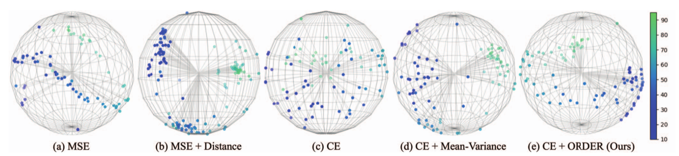
t-SNE of penultimate-layer embeddings on a sphere for MSE, MSE+Distance, CE, CE+Mean-Variance and CE+ORDER, coloured by age — Figure 3. t-SNE of penultimate-layer embeddings, coloured by age (10–95). MSE (a) is ordered but collapsed onto a thin band; cross-entropy (c) fills the space but scrambles the order; ORDER (e) keeps the space filled *and* ordered. From [1].

The remaining bias is asymmetric: SB-R (−2.5 y) is still larger than SB-L. Part of this is data, since the oldest tail of the cohort (ages 85–95) is thin even after oversampling; part is likely residual. The Neurology paper flags that no post-hoc correction was applied on top of ORDER, which is a deliberate choice but one to keep in mind when groups differ in age.

05 · Alzheimer's disease

Does \(\Delta_{\text{age}}\) order the AD continuum?

The frozen model was applied to 1,584 ADNI scans split by clinical trajectory: healthy controls (HC, n = 678), controls who later converted to MCI (HC→MCI, 179), stable MCI (432), MCI who converted to AD (139) and AD at baseline (156). Disease severity has a natural order HC < HC→MCI < MCI < MCI→AD < AD, so a good biomarker's group mean \(\Delta_{\text{age}}\) should follow it.

Table 4 · Mean \(\Delta_{\text{age}}\) (years) by ADNI clinical group, and Pearson correlation with severity rank (Table 4 in [1])
Loss	HC	HC→MCI	Stable MCI	MCI→AD	AD	Corr.
MSE	−1.2	−0.8	−0.3	+0.8	+1.5	0.98
MSE + Distance	−2.7	−1.9	−1.7	−0.9	+0.9	0.94
Cross-entropy	−1.9	−1.5	−3.4	−2.3	−4.1	−0.75
CE + Mean–Variance	−1.6	−0.3	−0.5	+0.8	+2.8	0.94
CE + ORDER (ours)	−1.5	−0.8	−0.3	+1.2	+2.0	0.98

Two things stand out. First, plain cross-entropy, despite a better MAE than MSE, is anti-correlated with disease severity (−0.75). Accuracy on healthy people is not sufficient; the feature space has to be ordinal for \(\Delta_{\text{age}}\) to mean anything off-distribution. Second, both MSE and ORDER reach r = 0.98, but with different group-pair statistics. ORDER separates AD from MCI→AD and shows a consistent monotone trend in pairwise significance, whereas MSE's pairwise map is disrupted (e.g. AD vs MCI→AD p = 0.16, AD vs stable MCI p = 0.56). For the pair that matters most for early detection, HC vs HC→MCI, ORDER gets p = 0.07 against MSE's p = 0.34.

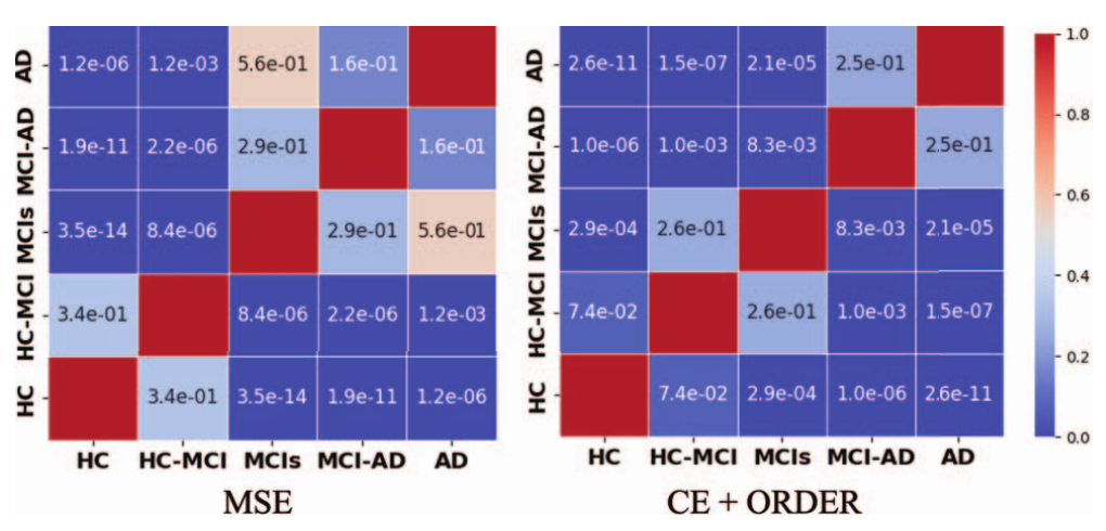
Heatmaps of pairwise t-test p-values between the five ADNI clinical groups for MSE and for CE+ORDER models — Figure 4. Pairwise t-test p-values on \(\Delta_{\text{age}}\) between the five ADNI groups. Blue is significant. The ORDER model (right) has a cleaner block structure along the severity diagonal than MSE (left). From [1].

Note that all group means are modest, within about ±2 years, and the HC mean is negative. The latter is expected since ADNI controls are a selected, well-screened group. What a biomarker needs is monotone ordering and separability between adjacent stages, and that is what the ordinal formulation buys. Our earlier regression-only analysis[6] (ADNI n = 1,175, ANCOVA controlling for sex, education and APOE4) had found the same ordering (F = 11.24, p < 0.0001) and already hinted that HC vs HC→MCI becomes significant when all visits, not just baseline, are used (p = 0.0009).

06 · Headache

Migraine, post-traumatic headache, and who recovers

Headache disorders affect roughly 40% of the global population and are, in the long run, associated with higher dementia risk, yet almost nothing is known about whether they alter brain ageing. Post-traumatic headache (PTH) after mild TBI is the sharper clinical problem: most people recover within three months, some progress to persistent PTH (PPTH), and there is no accepted way to tell them apart at the time of injury. The Mayo Clinic Arizona cohort let us ask both questions with the same frozen model[2,4].

Table 5 · Mayo Clinic AZ cohort and baseline \(\Delta_{\text{age}}\) (mean ± SE) [2]
Group	n	Age (y)	% female	\(\Delta_{\text{age}}\) (y)	vs HC
Healthy controls (HC)	137	39.5 ± 12.0	53.0	0.46 ± 0.87	—
Acute PTH (APTH)	99	42.2 ± 15.3	56.6	1.25 ± 0.87	p = 0.55
Migraine	93	39.6 ± 11.7	74.2	3.74 ± 1.03	p = 0.03
Persistent PTH (PPTH)	49	38.1 ± 10.6	34.7	4.65 ± 1.41	p = 0.01

One-way ANOVA across groups F = 3.53, \(\eta^2_p\) = 0.03, p < 0.05. APTH differed from PPTH (p = 0.04) and marginally from migraine (p = 0.08); migraine and PPTH did not differ (p = 0.67). Headache groups were diagnosed by ICHD-3 criteria. APTH participants were enrolled 0–59 days post-mTBI and had PTH for 30 ± 14 days before imaging; PPTH is PTH persisting beyond 3 months, here for about 11 years on average.

Bar chart of brain age delta in years for HC (0.46), acute PTH (1.25), migraine (3.74) and persistent PTH (4.65), with error bars — Figure 5. Baseline \(\Delta_{\text{age}}\) by headache phenotype. Controls sit near zero; migraine and persistent PTH brains look 3–5 years older than their chronological age; acute PTH is intermediate. From [2].2

The prognostic finding

The APTH group had prospectively collected headache diaries, so we could split it by outcome. Participants whose headache resolved before 3 months had a baseline \(\Delta_{\text{age}}\) of 1.28 ± 0.22 years. Those who had not recovered by 3 months: 1.63 ± 0.73. Those still symptomatic at 6 months: 3.46 ± 0.75, i.e. closer to the PPTH group than to controls, from a scan taken within weeks of the injury. The editorial that accompanied the paper[3] called this "the most clinically relevant finding of the study". It is also the one most in need of replication, because the 6-month group is small.

Where the model looks

Grad-CAM[16] on the age output, thresholded at the top 10% of voxels and mapped to the Desikan–Killiany atlas, gives a per-participant list of regions driving the prediction. We counted how often each region appears across participants in each group and kept those present in at least half. APTH and migraine each had about 20 such regions; PPTH had 12, all of which were shared with the other two groups. The signature is dominated by white matter, frontal above all, plus the basal ganglia.

Table 6 · Regions present in ≥ 50% of participants in all three headache groups (% of participants; Table 3 in [2])
Region	APTH	Migraine	PPTH
Right rostral middle frontal gyrus, WM	67.3	64.9	73.5
Left globus pallidus	61.2	59.6	69.4
Right postcentral gyrus, WM	61.2	59.6	63.3
Left lingual gyrus, WM	60.2	62.8	65.3
Right precentral gyrus, WM	58.2	64.9	53.1
Left isthmus cingulate, WM	58.2	62.8	51.0
Left precuneus, WM	56.1	60.6	51.0
Left superior temporal gyrus, WM	55.1	52.1	59.2
Left putamen	53.1	61.7	51.0
Right rostral anterior cingulate, WM	52.0	62.8	51.0
Left lateral orbitofrontal, WM	51.0	60.6	51.0
Left inferior parietal lobule, WM	51.0	57.4	57.1

Ten further regions (left caudate, right pars orbitalis WM, banks of the STS, paracentral, supramarginal, cuneus, …) met the threshold in APTH and migraine but not PPTH. Full list in [2].

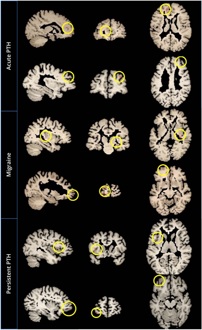
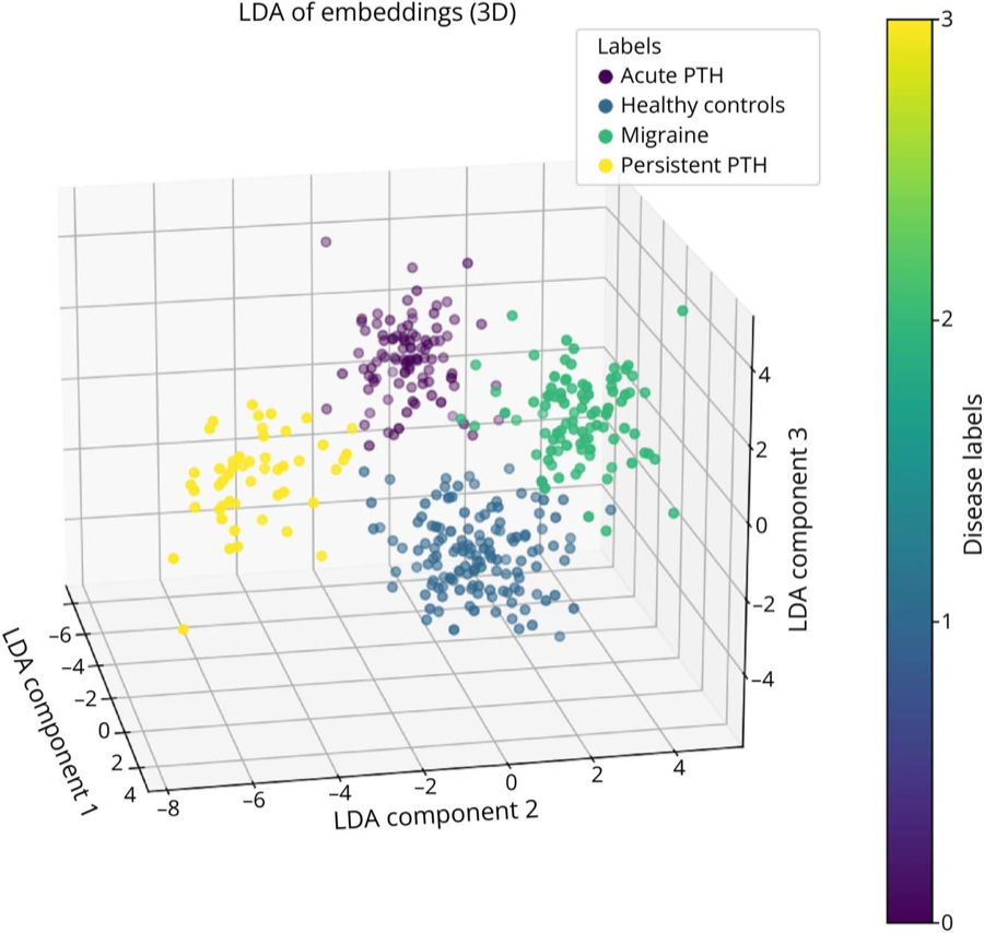
Grad-CAM peak activation regions circled on sagittal, coronal and axial T1 slices for acute PTH, migraine and persistent PTH participants — Figure 6. Peak Grad-CAM activations (≥ 50% of within-brain max) for randomly chosen participants per group. Only the single top activation is shown; Table 6 has the suprathreshold set. From [2].

3D LDA projection of penultimate-layer embeddings showing four clusters for healthy controls, acute PTH, migraine and persistent PTH — Figure 7. LDA of the 512-d embeddings. Four clusters follow the clinical labels (silhouette 0.60, Calinski–Harabasz 646, Davies–Bouldin 0.54). LDA is supervised, so this confirms label-driven structure rather than discovering it. From [2].

Two cautious readings. The regions are exactly the ones you would expect an age model to attend to: frontal WM loses volume with age, caudate and putamen are among the fastest-shrinking structures in normal ageing. That migraine and PTH register on those same features is the point, and the magnitudes line up with earlier reports of roughly +5 years after TBI[12] and +4 years in chronic migraine[13], but Grad-CAM tells us what made a brain look older, not what headache does to a brain. And the overlap between PTH and migraine is partly clinical: 76% of PPTH and 56% of APTH participants had migraine-like phenotypes.

07 · Perspective

"Accelerated ageing or biological vulnerability?"

The journal commissioned an editorial from Roberta Messina and Eduardo Caverzasi[3], and their framing is worth adopting. A single-timepoint \(\Delta_{\text{age}}\) is evidence of structural deviation from the normative trajectory, not proof of accelerated ageing per se; cross-sectional data cannot say whether the deviation precedes, accompanies or follows disease onset. They lay out three non-exclusive explanations for the elevated gap:

Consequence. Recurrent attacks drive structural change via hyperexcitability, neurogenic inflammation, oxidative stress or metabolic dysfunction. Our study cannot test this because we had no attack-frequency or disease-duration correlations.
Pre-existing trait. An older-looking brain predisposes to chronification. The APTH prognostic result is the evidence for this reading.
Shared cause. Both headache and elevated \(\Delta_{\text{age}}\) arise from a common process, e.g. impaired glymphatic function or altered cerebral energy metabolism.

Their anatomical observation is also sharper than ours: the signature sits in white-matter pathways and subcortical structures implicated in pain processing and sensory integration, not in the regions typical of neurodegeneration. On that basis they suggest elevated brain age "may be better viewed as a marker of biological vulnerability than as evidence of accelerated ageing itself", and that for now it is a research tool, not an individual-level clinical one. I agree with both.

08 · Caveats

Limitations and what comes next

Cross-sectional. Every clinical result above is from a single scan per person. The APTH group was imaged within weeks of injury and the PPTH group roughly a decade after, so persistence and time-since-injury are confounded. Longitudinal imaging is the obvious next experiment and the one both we and the editorial ask for.
Sample sizes. PPTH n = 49, and the 6-month-persistent APTH subgroup is smaller still. The effect sizes are plausible but the confidence intervals are wide.
Residual bias. ORDER reduces regression to the mean; it does not eliminate it (SB-R = −2.5 y). Group comparisons were not covariate-adjusted for age, sex or education, and no post-hoc correction was applied. Groups here are age-matched (all about 40 ± 12 y), which limits the damage, but a confirmatory analysis should do both.
Unmeasured confounders. Cardiovascular risk, white-matter hyperintensities, cognitive status, medication, and whether the person was mid-attack during the scan were not available.
Normative data. Public lifespan cohorts were not screened for headache, so some "healthy" training subjects were likely migraineurs. This biases the norm toward older-looking brains and makes our group differences conservative, not inflated.
Interpretability. Grad-CAM is exploratory and prone to false positives and negatives when many regions contribute at once. Occlusion sensitivity, Integrated Gradients or SHAP-style attribution would be the right cross-check.

Methodologically, the ORDER idea is not specific to brains or to age. Any regression problem with an ordinal target and a suspected regression-to-the-mean problem can be posed this way, and the ordinality metric gives a cheap diagnostic for whether a learned feature space actually respects the order you care about. That generalisation is something I would like to see tested beyond neuroimaging.

References

Papers, slides and code

J. Shah, M. M. Rahman Siddiquee, Y. Su, T. Wu, B. Li. Ordinal Classification with Distance Regularization for Robust Brain Age Prediction. Proc. IEEE/CVF WACV, 2024. paper arXiv pdf code
J. Shah, G. Dumkrieger, C. D. Chong, T. J. Schwedt, T. Wu. Advanced Brain Aging Associated With Migraine and Posttraumatic Headache: A Deep Learning Study. Neurology Open Access, 2026;2:e000158. doi:10.1212/WN9.0000000000000158 pdf
R. Messina, E. Caverzasi. Brain Age Prediction in Migraine and Posttraumatic Headache: Accelerated Aging or Biological Vulnerability? Editorial. Neurology Open Access, 2026;2:e000173. doi:10.1212/WN9.0000000000000173 pdf
J. Shah, M. M. Rahman Siddiquee, C. D. Chong, T. J. Schwedt, J. Li, V. Berisha, K. Ross, T. Wu. Capturing MRI Signatures of Brain Age as a Potential Biomarker to Predict Persistence of Post-traumatic Headache. Oral presentation, American Academy of Neurology Annual Meeting, 2024. abstract slides
J. Shah, J. Luo, J. Sohankar, E. M. Reiman, K. Chen, Y. Su, B. Li, T. Wu. A Multi-class Deep Learning Model to Estimate Brain Age While Addressing Systematic Bias of Regression to the Mean. Alzheimer's Association International Conference, 2023. doi:10.1002/alz.082691 pdf
J. Shah, V. Ghisays, Y. Chen, J. Luo, B. Li, E. M. Reiman, K. Chen, T. Wu, Y. Su. MRI Signatures of Brain Age in the Alzheimer's Disease Continuum. Alzheimer's Association International Conference, 2022. doi:10.1002/alz.061942 pdf
J. Shah. Novel Deep Learning Techniques for Early Detection of Neurological Disorders. Ph.D. dissertation, Arizona State University, 2025. Chapter 3, Robust Brain Age Prediction. doi:10.6084/m9.figshare.31768441.v1 defense slides
K. Franke, G. Ziegler, S. Klöppel, C. Gaser. Estimating the age of healthy subjects from T1-weighted MRI scans using kernel methods: exploring the influence of various parameters. NeuroImage, 2010;50(3):883–892.
S. Zhang, L. Yang, M. B. Mi, X. Zheng, A. Yao. Improving Deep Regression with Ordinal Entropy. ICLR, 2023.
H. Pan, H. Han, S. Shan, X. Chen. Mean-Variance Loss for Deep Age Estimation from a Face. CVPR, 2018.
J. H. Cole, S. J. Ritchie, M. E. Bastin, et al. Brain age predicts mortality. Molecular Psychiatry, 2018;23:1385–1392.
J. H. Cole, R. Leech, D. J. Sharp. Prediction of brain age suggests accelerated atrophy after traumatic brain injury. Annals of Neurology, 2015;77(4):571–581.
R. Navarro-González, D. García-Azorín, Á. L. Guerrero-Peral, et al. Increased MRI-based brain age in chronic migraine patients. Journal of Headache and Pain, 2023;24:133.
H. Liang, F. Zhang, X. Niu. Investigating systematic bias in brain age estimation with application to post-traumatic stress disorders. Human Brain Mapping, 2019;40(11):3143–3152.
C. C. Aggarwal, A. Hinneburg, D. A. Keim. On the surprising behavior of distance metrics in high dimensional space. ICDT, 2001.
R. R. Selvaraju, M. Cogswell, A. Das, R. Vedantam, D. Parikh, D. Batra. Grad-CAM: Visual explanations from deep networks via gradient-based localization. ICCV, 2017.